Working with Colours
Since the release of version 8 of PTV Viswalk, it has been possible to assess the density in the immediate vicinity of individual pedestrians, and to display this data on the pedestrians themselves using colour coding. Even before this development it was also possible to visualise certain other static and dynamic values in this way, including:
- Pedestrian type
- Starting area
- Destination of the current route
- Distance to next (intermediate) destination
- Current speed
Both the current speed and the experienced density can be aggregated over time and displayed on the cells of a grid.
In this post we will discuss how to configure this functionality in PTV Viswalk 8 and explain the difference between ‘experienced density’ and ‘density’ when displayed on the grid cells.
Colour-coding pedestrians
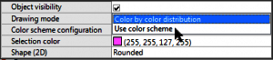
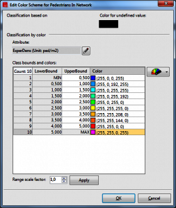
You can access the colour-coding function via the graphics parameters under Pedestrians in Network, regardless of which value you wish to colour code. Change the Drawing mode to Use colour scheme. Then select a classification attribute in the dialogue box that opens.
 |  | 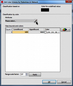 |
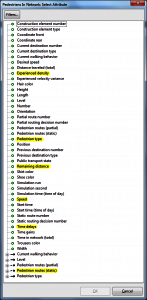
You can choose from a range of classification parameters (all attributes applied to the pedestrian, plus attributes of objects linked to the pedestrians such as routing decisions and routes). Of course, it would not for all of these parameters make sense to be used for colour-coding pedestrians. Here, we have highlighted the parameters that were used in the video. Next, you need to define useful classes and assign colours to these. The new configuration is indicated on the network object page list in the graphic parameters icon.
 |  |  |
As a side note: The colour-coding of vehicles in Vissim can also be configured in the same way.
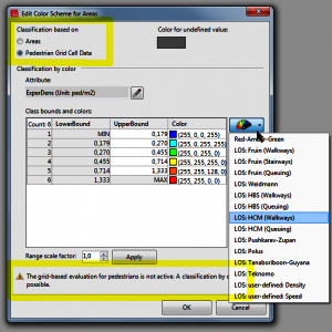
The area colour-coding can be configured in a similar way via the area (and ramp) graphics parameters. However, you also need to decide whether to base the classification on areas or on grid cell data. You must also activate the “Areas and ramps” entry under [Evaluation] → [Configuration] → Result attributes (and if necessary specify the size of the measurement area under [More…]) in order for the required data to actually be collected.
Experienced density vs. density
When you configure the classification for the areas or grids, you may notice that you have the option to select ‘Density’ as well as ‘Experienced density’. What is the difference? You can clearly see in the video on youtube that each value leads to obvious differences:
The difference lies in the perspective. As the name suggests, Experienced density measures the density within the immediate vicinity of each individual pedestrian, and is available as a dynamic attribute for each pedestrian – just like the speed of each pedestrian. Incidentally, the grid cells can also be colour-coded based on pedestrian speed. The size of the area around a pedestrian within which the density should be measured can be configured in [Base Data] → [Network Settings] → “Pedestrian Behavior”. This is set to 2 metres by default. In order to make this density calculation completely subjective, the pedestrian concerned is not included in the calculation of its own experienced density. During each time interval of the simulation, the grid cells access the experienced density values available for those pedestrians who in that moment are located in its immediate surroundings, and at the end of the time interval they use these values to calculate an average value that is then displayed by means of colour-coding.
By contrast, the perspective of an external observer is assumed when calculating the Density. The number of pedestrians on a grid cell or in its immediate vicinity is calculated, and this is divided by the corresponding content of the area.
The fundamental difference lies in the averaging process during the time period under consideration. For Experienced density, the total of the individual measurements for each pedestrian is divided by the number of measurements at the end of the time interval for each grid cell. This means that high density values inevitably receive a heavier weighting on average than smaller density values: On the one hand, there is no value for the individual time step, and no value is contributed to the measurement result for time steps in which there are no pedestrians in the immediate vicinity of the grid cell (although the value 0 is still possible if a pedestrian experiences a subjective density of 0). On the other hand, it contributes a large number of values for time steps in which there are many pedestrians located within the vicinity of a grid cell.
By contrast, when calculating the average time interval value for Density, just one value is calculated for each time step and this value is averaged over all time step values. This means that all density values are treated equally, regardless of whether those values are large or small. As a result, small density values are taken more into account (relative to large density values) than they are in experienced density. However, the average values for density are not always higher than those for experienced density, as the individual pedestrian from whose perspective the experienced density is calculated is not taken into account in the calculation of experienced density.
To use a visual metaphor: density describes how carpets are worn away, as well as giving the same overall impression as that enjoyed by a station operator or factory supervisor watching flows of people on a monitor. Experienced density, by contrast, corresponds to the results you might expect from a survey, or to what you might find in customer letters or social media posts.
Naturally, we need to decide which of the two measures is the correct or more relevant one. If you need to pick one of the two, then you should choose experienced density, as the subjective experiences of customers and visitors are highly relevant to operators. However, because operators are normally also responsible for maintaining an external perspective on events, a combination of both values should be used. If the density distribution display resulting from the simulation corresponds to the perspective of an external observer, this increases users’ confidence in the accuracy and relevance of the experienced density display. Ultimately, it is not necessary to decide between the two displays; you can switch back and forth between them instead.
Video production
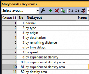
Finally, it should be noted that the videos edited together under the link can be recorded within a single simulation run. In order to do this it is necessary to define the corresponding layouts in the network editor and to use these in the individual storyboards.